Welcome to the second post of the blog series I am writing on Azure Synapse Analytics. As you know Azure Synapse Analytics went GA December of 2020, and in the following blogposts I would like to walk you through the out-of-the-box capabilities you have to report easily on a vast dataset.
Azure Synapse Analytics series
- Azure Synapse Analytics – Serverless SQL Pools
- Azure Synapse Analytics – Serverless SQL Pools: Partitioning
- Azure Synapse Analytics – Serverless SQL Pools: Data Elimination
Setting the stage
In this blogpost we will again be using the TLC taxi dataset which contains over 1.4B rows.
In Today’s post I would like to show you how you can optimize your queries built by Serverless Synapse SQL Pools by partitioning your data. I will start by giving a bit of background on how Serverless SQL Pools handle queries in the background and tell you how partitioning fits in here.
Serverless SQL Pools has decoupled not only compute and storage, but it has also decoupled state. Decoupling state means that we are no longer depended on a compute node failure, which is the key difference with stateful architectures. The compute nodes in Serverless SQL Pools do not hold any state information, this allows it to partially restart queries in an event of a node failure AND This will also allow us to scale out without impacting any running transactions.
Another thing that makes the engine unique is that each compute node will be based on the SQL Engine which will then optimize the local data handling through the cost-based SQL System and help with scaling up the compute nodes.
This gives the Serverless SQL Pools the ability to not only scale-out, but also to scale-up nodes!
When a query gets send, what Serverless SQL Pools does, is create a logical list of “cells” from a dataset, these cells are then used to achieve parallelism by assigning them to multiple compute nodes. The data extraction of a cell is the responsibility of a single node, which is a SQL Server in the background.
The mapping of the “cells” to the compute for query execution is achieved through hash distribution, this will map the different distributions(“cells”) to compute nodes. With proper distribution, we can avoid data movement for the group by columns or join clause columns.
Data movement (Intermediate Steps) between compute nodes will slow down queries and is what we want to avoid. So, the Distribution of your data is key to having a fast-performing Serverless SQL Pool (Same as Stateful SQL Pools btw).
Next to distribution, we can also benefit from partition elimination by partitioning the data on equality or range predicates.
The Distribution and Partitioning strategy will allow the Serverless SQL Pools to reduce the amount of read action to the dataset and selectively reference grouping of “cells’ or single “cells” depending on the query you write.
Today’s post will focus on the partition elimination using range predicates or equality predicates on a parquet source.
Partitioning data
The dataset I used in the previous blog were parquet files located in a single folder without using any partitioning.
This means that we would not be able to benefit from partition elimination to optimize the queries we are using in our report. When we are not leveraging partitioning, queries will be slower, read more data and will also be more expensive.
I will start by partitioning my data by each year.
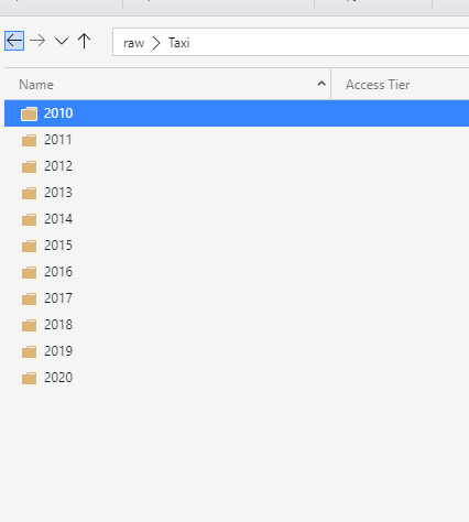
As you can see in the image above, I created a folder for each year and in those folders the data will reside for that specific year.
I will now create a new view in the ServerlessTaxi database I created in the previous blogpost, this view will reference the new partitioned parquet structure. I will be using a specific functionality for the openrowset which is called FilePath.
CREATE VIEW dbo.TaxiYearPartitioned
as
SELECT *,
cast(Taxi.filepath(1) as varchar(4)) as Year
FROM
OPENROWSET(
BULK 'https://xxx.dfs.core.windows.net/raw/Taxi/*/*.parquet',
FORMAT='PARQUET'
)
WITH
(
Passenger_Count int,
Trip_Distance float,
store_and_forward bit,
Payment_Type int,
mta_tax numeric(10,2),
VendorID int,
PULocationID int,
DOLocationID int,
tpep_pickup_datetime datetime,
tpep_dropoff_datetime datetime,
RatecodeID int,
Fare_amount numeric(10,2),
Extra float,
Tip_amount numeric(10,2),
Tolls_amount numeric(10,2),
Total_amount numeric(10,2),
improvement_surcharge numeric(10,2),
congestion_surcharge int,
PickupDate date,
DropoffDate date
)AS [Taxi]
Filepath(1) here specifies the first * in the folderpath of my openrowset which is the foldername containing the year, if I would like to specify the second part which would be the filename, I would have to write Filepath(2).
Reporting Impact
After creating this view, I would like to see what impact this would make on queries in my report using that year column.
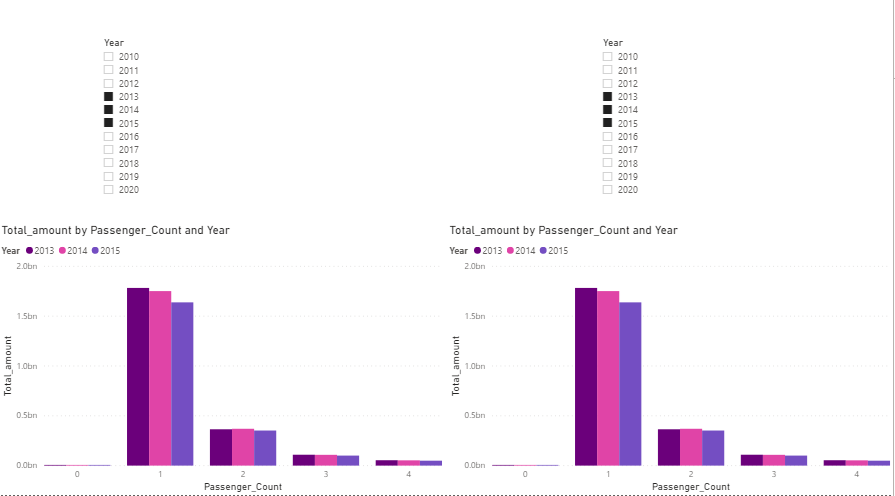
I will start by creating a new Power BI Report. I will use Direct Query to get taxi dataset view unpartitioned and the taxi dataset partitioned by year. The unpartitioned dataset is a new view which has the year() function in there to fetch the year from the tpep_pickup_date.
On these two datasets I will create a year slicer for each dataset, and I will create a line graph showing me the number of sales by year and amount of passengers.
This is the small dashboard I build. The left side is the unpartitioned and the right side is the partitioned.
I opened up the performance analyzer and ran the refresh of the visuals.
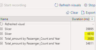
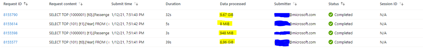
The difference with the partitioned view is quite big, as for the year function we will need to analyze almost all of the data, while the partitioned data is able to just scan the partitions we want data from. This translates into the following queries in the query monitor in the Synapse Workspace.
Conclusion
By partitioning the data of the Taxi dataset, we can drastically reduce the amount of data being read. This minimizes the cost when running this specific report.
This will also give us a drastic performance increase as we can filter the number of “cells” pushed to compute.
In this specific case we read only 10% of the data when loading the graph, and almost read no data when loading the slicer. Next to this we reduced the query runtime to 10% of the original which are great performance improvements!
The filepath option you have in openrowset allows you to effectively tune your datasets, as this is not limited to one level, we can possibly create multiple partitioning layers and optimize queries even further.
This concludes this blogpost on Serverless SQL Pools and Partitioning, in the next blog of this series we will be talking about modeling your data with Serverless SQL pools.
Thank you for reading and stay tuned!
![]()